Determinants of the Optimal Waste Disposal Charge Rate: A Numerical Simulation with Comparative Statics
Abstract
This study examines the factors determining the socially optimal disposal charge rate under Korea’s final waste disposal charge system. Comparative static analysis and numerical simulation are employed to determine the relative importance of unit external costs, market structure, and market elasticity. The waste treatment service market is modeled as an imperfectly competitive market that includes perfect competition as a special case, and market structure is explicitly treated as an independent parameter, alongside unit external costs and elasticity. Waste generators and treatment service providers maximize their profits, whereas the social planner aims to maximize social welfare. The optimal disposal charge rate is defined as the rate that maximizes social welfare, levied on waste generators in proportion to the amount of final disposal. The comparative static derivatives for each parameter are derived using a system of equations based on the first-order conditions that satisfy both profit maximization and market equilibrium. As the signs and approximate magnitudes of the derivatives alone are insufficient for policy decisions, numerical simulations are used to compare and quantify the relative importance of each parameter. The results reveal that in a competitive market, the optimal disposal charge rate is determined solely by the unit external cost, with market elasticity having no effect. Contrastingly, under imperfect competition, all three parameters affect the optimal rate—market structure has the greatest effect and is followed by unit external cost, whereas market elasticity has the least effect. The policy implications are as follows: (1) information on market structure is crucial in determining the optimal disposal charge rate, as it significantly affects the influence of other parameters; (2) decision-making based on market elasticity is irrelevant in competitive markets and may diminish welfare under imperfect competition; and (3) unit external cost is pivotal in both competitive and imperfectly competitive markets
초록
본 연구는 폐기물 최종처분 부담금 제도의 시행에 있어 사회적으로 최적인 부담금 요율을 결정하는 데 영향을 미치는 요인을 분석하였다. 이를 위해 비교 정태 분석과 수치 시뮬레이션 방법을 적용하였으며, 분석 대상 파라미터로는 단위 외부 비용, 시장구조, 시장 탄성치를 포함하였다. 폐기물 처리 서비스 시장을 완전 경쟁을 포함한 불완전 경쟁 시장으로 설정하고, 시장구조, 탄성치, 단위 외부 비용 등을 명시적인 파라미터로 고려하였다. 폐기물 배출자와 처리업자는 이윤 극대화를 추구하고, 사회 계획가는 사회 후생 극대화를 목표로 하여 최적의 처분 부담금 요율을 결정한다. 비교 정태 도함수는 이윤 극대화 조건과 시장균형 식을 만족하는 조건식들로 이루어진 방정식 체계로부터 유도되었으며, 도함수의 부호와 대략적 크기만으로는 정책 판단에 한계가 있어 수치 시뮬레이션을 통해 파라미터의 상대적 중요성을 정량적으로 비교하였다. 분석 결과, 경쟁 시장에서는 단위 외부 비용만이 최적 요율 결정에 영향을 미치며, 시장 탄성치는 영향을 미치지 않았다. 반면, 불완전경쟁 시장에서는 세 가지 파라미터 모두가 영향을 미치며, 이 중 시장구조의 중요성이 가장 크고, 그다음으로 단위 외부 비용과 시장 탄성치 순으로 중요한 것으로 나타났다. 정책적 시사점으로는, 첫째, 시장구조는 다른 파라미터에 대하여서도 영향을 미치므로 그에 대한 정보가 매우 중요하며, 둘째, 시장 탄성치에 의존한 최종처분 부담금 요율 결정 방식은 경쟁 시장에서는 무용하고 불완전경쟁시장에서는 후생을 저하할 가능성이 있으며, 셋째, 단위 외부 비용은 경쟁 시장뿐 아니라 불완전경쟁시장에서도 중요하다는 것이다.
Keywords:
Market Structure, Waste Treatment Service Market, Optimal Disposal Charge Rate, Comparative Static Analysis, Numerical Simulation, Elasticity, Unit External Cost키워드:
시장구조, 폐기물 처리 서비스, 시장 최적 처분부담금 요율, 비교정태분석, 수치 시뮬레이션, 탄성치, 단위 외부 비용Ⅰ. Introduction
1. The Background: Waste Disposal Charge System in Korea
In Korea, the Framework Act on Resource Circulation came into effect in 2018. This Act includes the clauses for Waste Disposal Charge System. Korea’s Waste Disposal Charge System is designed as follows. Municipalities or business waste emitters are levied 10~30 KRW/kg for landfill and 10 KRW/kg for incineration of wastes. When the one who should pay the charge recycles the wastes in three years or he/she recovers the heat energy more than 50%, it is exempt. Small businesses are lessened or exempt for the charges. Designated wastes which are very difficult to recycle, wastes in islands, wastes from disaster area are eligible for exempt or reduced charges. Revenues from the charges are used to promote the social recognition for resource circulation, to support for small scaled resource circulation facility, to help classified collection of wastes, and to support the production and distribution of circular resources and recycled products.
2. Objective of the Study
Although the Waste Disposal Charge has been in practice since 2018 in Korea, there is a room for controversy on whether the charge rate is designed close enough to the optimum. Despite that the fundamental principle of economics teaches waste disposal charge should reflect externality, in reality, the decision makers in the governments do not seem to consider unit external cost as the single most important factor that determines the environmental tax rate or disposal charge rate. Elasticity is sometimes used as an important parameter, occasionally considered even more important than the unit external cost. The market is usually assumed competitive, implicitly or explicitly, even though in reality the market is often in an imperfect competition. In practice, neither of these factors are seriously considered because there is no sufficient information on the unit external cost, market elasticity, or market structure. In many cases the expected or desired revenue seems to be the most important consideration to the decision making government authorities. Maybe this is the reason why policy makers are sometimes concerned with elasticity while market structure or unit external cost are not seriously considered.
This paper attempts to provide explanations on this question using comparative statics and numerical simulations with a model built on the waste treatment services market. The motivation of this study is to answer the following questions: 1) How should we determine the optimal disposal charge rate?, 2) How much do the external cost of final disposal, elasticity, and market structure matter?, and 3) What are the policy implications?
3. Related Previous Studies and Their Implications for This Study
In standard environmental economics textbooks, optimal environmental tax rate is unit external cost in a competitive product or environmental service market. However, when the market is in imperfect competition, optimal environmental tax rate differs from unit external cost. Studies on the optimal environmental taxes in imperfectly competitive markets are focused either on a product market or environmental services market.
There are many studies focusing on product markets. Misolek (1980), Barnett (1980) and many other studies posit that when polluting industry is monopoly, the optimal environmental tax rate will be lower than the one for competitive case. Requate (2005) reaffirms that with monopoly the optimal tax rate is lower than Pigiouvian tax rate. Requate (2005) also showed that in oligopoly optimal environmental tax rate decreases with the increase in the number of symmetric firms. This is equivalent with the statement that lower market concentration reduces the optimal environmental tax rate. Bovenberg and Gould (1996) state that if there are taxes other than environmental tax, the optimal environmental tax rate is lower than the external cost. Sandmo (1975) showed that the optimality of the Pigouvian tax can be achieved by adjusting the indirect tax system when an environmental tax is implemented as an element in a more comprehensive indirect tax system. However, this does not refute the fact that the optimal tax diverges from the Pigouvian tax if other taxes still exist. Kim and Kim (2002) showed that when a tax on capital exists, the optimal environmental tax rate is lower than the environmental externality cost. Lho (2002) introduced a generalized utility function and constructed a model in which citizens maximize utility as a function of consumption, leisure, and environmental pollution, and environmental pollution occurs from consumption. By using this social utility function, the optimal environmental tax rate is numerically derived by given specific values of parameters. In addition, a sensitivity analysis is conducted on the optimal environmental tax rate over the various values of parameters. From the numerical simulation and sensitivity analysis, Lho (2002) showed that the optimal environmental tax rate is a decreasing function of the concavity parameter of the social welfare function and an increasing function of the elasticity of substitution of leisure and final consumer goods.
There are a few studies focusing on environmental services market. Baumol (1995) and Feess and Muehlheusser (1999, 2002) acknowledged the existence of the eco-industrial sector, but they did not explicitly address the consequences of imperfect competition on the optimal environmental tax rate. David and Sinclair-Desgagné (2005) analyzed the optimal pollution tax when pollution abatement technologies and services are provided by an imperfectly competitive environment industry. They found that under endogenous market elasticity, the optimal pollution tax will be higher than the marginal social cost of pollution. David, Nimubona and Sinclair-Desgagné (2011) examined the effect of emission taxes on pollution abatement and social welfare, where abatement goods and services are provided by a Cournot oligopoly with free entry. They showed that under endogenous market structure, it is highly probable that the welfare maximizing emission tax is lower than the simple Pigouvian tax. 1)
There are fewer studies regarding environmental tax in waste treatment service market. Kaneko (2009), using a partial equilibrium comparative statics model based on a vertically linked competitive waste treatment services markets, demonstrated that the waste generation reduction effect differs by the point of levying industrial waste tax. However, Kaneko (2009) did not provide the welfare implication of these tax options.
Kim and Chang (2015) calculated potential environmental benefits (with a given unit external cost) and tax revenue from Korea’s final disposal charge by conducting simulations, apparently with the assumption of a competitive market. Elasticity is considered as the major factor in determining the charge rate for final disposal in Kim and Chang (2015), without explicitly considering social welfare.
4. Characteristics of This Study Demarcating from Previous Studies
Adding to the unit external cost, which is the starting point and basic element in determining the optimal disposal charge rate, several studies have examined additional factors. Barnett(1980), Requate(2005) and others suggested the role of market structure in optimal disposal charge rate. Kim and Chang (2015) demonstrated the importance of elasticity. Kaneko(2019) showed the importance of considering levying method in designing the charge schemes. David et al.(2011) analyzed the optimal environmental tax rate in the oligopolistic environmental service firms, and Lho (2002) applied a numerical simulation method to a social utility function to derive the optimal environmental tax rate.
This study aims to identify the relative importance of the determinants of the optimal waste disposal charge rate. This can be achieved by synthesizing various elements of previous studies and adding new ones. Those characteristics differentiating this study from previous ones are as follows. First, assuming a generalized imperfectly competitive market, the market structure is expressed in a continuum from perfect competition to pure monopoly/monopsony, so we can parameterize the market structure for buyer’s and seller’s side. Hence, now we have three parameters of market structure, market elasticity, and unit external cost. Second, compared to previous studies that analyzed products or input markets, this study is focused on the waste treatment service market so that the market structure and elasticity in the waste service sector are explicitly considered so the policy implications are more appropriate to the environmental policy practitioners. Third, by conducting comparative statics and numerical simulations, it is possible to compare the relative size of the impact of the different parameters in determining the optimal disposal charge rate. This is an improvement compared with the previous studies.
Ⅱ. The Model for Comparative Static Analysis and the Results
1. Definition of Variables, Structure of the Waste Treatment Service Market, and Objective Functions
Waste generators generate constant amount of waste . Waste generators have two choices in dealing with the generated waste. The first choice is to transfer the waste to the waste treatments service providers 2) by the amount of w. In this case, the waste treatment service providers receive fee of p per quantity of waste delivered. The value of p is determined in the market. The second choice is waste reduction. 3) The quantity of waste reduction, which is the quantity of waste not delivered to the waste treatment service providers, is e-w. The cost incurred in the process of reduction is a function of e-w, denoted CE(e-w). 4)
The cost of waste treatment is a function of w, denoted CT(w), which includes the costs of collection, transportation, pre-treatment, treatment, and final disposal. Waste disposal charge (t per quantity of waste disposed) is to be levied on the final disposal and paid by the waste generators. 5)
Waste generators’ problem is maximizing profit by choosing w, given constant e and market-determined variable p. Waste generators’ cost is the sum of waste reduction cost CE(e-w) plus the payment to waste treatment service providers pw. 6) So waste generators’ profit maximization problem becomes in fact a cost minimization problem.
Waste treatment service providers, after receiving w from waste generators, provide waste treatment services and finally dispose wastes. Waste treatment service providers receive pw as revenue for their services and incur treatment cost of CT(w). 7) Waste treatment service providers maximize profits by choosing w, given p that is determined in the market.
These relationships are depicted in the following <Figure 1>.

Flow of Service and Money in the Waste Treatment Service Market
2. Parameters of Market Structure, Market Elasticity, and Externality
In the model, we have variables w and p and a constant e, as well as several parameters for elasticity, market structure, and environmental externality. The objective of this study is to assess and compare the relative importance of three parameter groups of unit external costs, market structure, and market elasticity in determining the optimal charge rate for the final disposal of wastes.8)
Regarding market elasticity, we have parameters g of h and . The slope of marginal cost function of waste reduction , CE"(e-w), which is the minus of the slope of market demand curve of the waste treatment service, 9) assumed to be a non-negative constant, is denoted g as a parameter for the inverse of demand elasticity. The slope of market supply curve of waste treatment service, which is CT"(w)10), assumed to be non-negative constant, is denoted h as a parameter for the inverse supply elasticity. The condition for the inverses of slopes of the demand and supply curves to be elasticity is that the price and quantity are assumed to normalized to unity at the equilibrium. In this study, price (p) and quantity (w) of waste treatment services are assumed to be unities at the equilibrium.
Regarding externality, the unit external cost of final disposal is denoted θ. Regarding market structure, the uniform market share is βg for waste service provider (seller of the service) and βh for waste generator (buyer of the service) , where 0≦βg≦1 and 0≦βh≦1. 11)
This study assumes the market is in an imperfect competition (Cournot oligopoly and oligopsony). Following Appelbaum(1982). Ji and Chung(2016), and Chung(2017), in an imperfectly competitive oligopoly/oligopsony, when the market is composed of uniformly sized firms, the market power or Lerner index is expressed as , where β is the market share for uniform firms and η is the elasticity for demand or supply. 12) In other words, the market power of individual firms is the market share of each uniform firm (market structure parameter) multiplied by the reciprocal of market elasticity.
In this study, market elasticity is assumed to be the reciprocal of the slope of the demand or supply curve at the equilibrium. 13) Therefore, we have the equations for the market power of individual sellers and buyers, , where g is the slope of the demand curve and h is the slope of supply curve, and βg is seller’s market share and βh is buyer’s market share, ηg is market elasticity of demand and ηh is market elasticity of supply. Please remind that demand curve slope represents the seller’s market power and supply curve slope represents the buyer’s market power, not the other way around. Also remind that market demand or market supply curve is different from the demand curve faced by individual sellers or the supply curve faced by individual buyers.
Market power of individual sellers or buyers is equal to the inverse of elasticity of demand or supply faced by individual sellers or buyers, which is seller’s or buyer’s market share divided by demand or supply elasticity. Market power of individual sellers or buyers, which is inverse of elasticity of demand or supply faced by individual sellers or buyers, is proportional to the market share. In this study, the inverse of elasticity is the slope of demand or supply curve. Hence, the slope of demand or supply curve faced by individual sellers or buyers is proportional to the market share. The slope of the demand curve faced by individual sellers is seller’s market share times the slope of market demand curve (βgg). The slope of the supply curve faced by individual buyers is the buyer’s market share times the slope of the market supply curve (βhh).
3. Behaviors of market participants and social planner
The objective of waste generators is profit maximization regarding waste related activity. Non-waste related variables assumed to remain constant. In addition, the quantity of waste generated is also assumed to be constant. Therefore, the profit maximization for waste generator becomes equivalent to the minimization of waste related costs. Waste generators’ objective is minimizing the sum of cost of waste reduction, waste treatment fee paid to the waste treatment service providers, and disposal charge paid to the government.
Waste reduction cost is a function of (e-w), that is CE(e-w). Treatment fee is the product of fee rate and the quantity of waste transferred, pD(w). Here pD(w) is buyers’ (waste generators’) ex-ant offer price for the waste treatment services, i.e., inverse demand function of waste treatment services. The value of disposal charge paid to the government is tw where t is the disposal charge rate.
Waste treatment service providers are maximizing profit, which is the revenue from waste treatment service minus the cost of waste treatment. Revenue from waste treatment service is pS(w), where pS(w) is sellers’ (waste treatment service providers’) ex-ant offer price of waste treatment services, i.e., inverse supply function of waste treatment service. We have pD(w) = pS(w) in equilibrium.
Given profit maximizing behaviors of the market participant and the market equilibrium condition, the social planner maximizes the social welfare. The social planner maximizes the social welfare after observing the profit maximizing behaviors of waste generators and waste treatment service providers.
Behaviors of waste generators and waste treatment providers are given as follows.
| (Equation 2) |
Since the social planner determines the optimal disposal charge rate after observing the behaviors of market participants given a disposal charge rate, the sequence of obtaining the optimal disposal charge rate is as follows.
By getting the first order conditions for the waste generator and the waste treatment service provider regarding w, and combined with the equilibrium condition, we get the followings.
| (Equation 3) |
Since , and , we get the followings, 14).
| (Equation 16) |
The Stackelberg condition is satisfied by considering w as a function of t. Hence the social planner’s problem is as follows.
| (Equation 17) |
By getting first order condition regarding t from (Equation 4), we get , we get –gw–hw–θ=0
So we have the following three equations with three variables w, p, and t. 15)
| (Equation 18) |
4. Comparative statics results and discussions
By applying the implicit function rule for the previous equations in (Equation 5), we get the following results for comparative static derivatives regarding the impact of parameters on the optimal disposal charge rate. 16)CE'
| (Equation 19) |
First, θ is the unit external cost and is the impact of unit external cost on the optimal disposal charge rate. Second, g is minus of the slope of demand curve, which measures the inverse market elasticity of demand, where is the impact of inverse market elasticity of demand on the optimal disposal charge rate. Third, h is the slope of supply curve, which measures the inverse market elasticity of supply, where is the impact of inverse market elasticity of supply on the optimal disposal charge rate. Fourth, βg is seller’s market share., where is the impact of seller’s market share on the optimal disposal charge rate. Fifth, βh is buyer’s market share., where is the impact of buyer’s market share on the optimal disposal charge rate.
Regarding the impact of unit external cost, we obtained . It is assumed that 0≤βg,βg≤1. When both the sellers and buyers are competitive, or when both sellers’ market share (βg) and buyers’ market share (βh) are zeroes, then =1. When the seller is in pure monopoly and and buyer is in pure monopsony, or both seller’s market share (βg) and buyer’s market share (βh) are unities, then will be 2. Therefore, we have an inequality 2≥≥1. When the market is competitive both in the seller’s and buyer’s side, the optimal charge rate for waste disposal is proportional to the unit external cost, and in most cases the optimal charge rate is identical to the unit external cost. The value of increases with the sellers’ or buyers’ market share increases. This implies the importance (sensitivity) of the unit external cost in determining the optimal charge rate increases as the market power of sellers or buyers increases. It is quite remarkable that although market powers make the optimal disposal charge rate lower, 17) the sensitivity of optimal disposal charge rate to the unit external cost increases as market powers increase.
We have parameters related to elasticity, g and h. g is minus of the slope of market demand curve, which is equal to the inverse of market demand elasticity under the assumption of price of the waste treatment service p=1 and quantity of service w=1. h is the slope of market supply curve, which is equal to the inverse of market demand elasticity under the assumption of p=1 and w=1.
We denote βg-βh as βGAP. Regarding inverse demand elasticity, it is found that , and regarding supply elasticity, it is found that . The signs are indeterminate depending on the sign of βGAP.
Demand elasticity or supply elasticity does not matter at all to the optimal charge rate when the buyers and sellers have symmetric market shares, which means βGAP=0. Symmetric market shares include the case of perfect competition where βg=βh=0 . In an imperfectly competitive market with asymmetric market shares, which means βGAP≠0, demand or supply elasticity matters to the optimal charge rate. However, because the signs are dependent t on the sign of βGAP, the direction of the effect of elasticity to the the optimal charge rate is indeterminate.
It is found that . Since g and h are non-negative and w is equal to 1, . These results state that higher market share of seller or buyer results in lower optimal disposal charge rate. 18) This is in line with the results from previous studies (Barnett(1980) and others) that posits the optimal environmental tax rate is lower in a monopoly than in a competition.
In addition to the market share’s importance by itself, it is also notable that the impacts of market elasticity and unit external cost on the optimal disposal charge rate also depend on the market shares. That is, market share plays a role in determining the size of the impact of unit external cost or elasticity on the optimal waste charge rate. Higher market share makes the optimal charge rate more sensitive to unit external cost. The gap between seller’s and buyer’s market concentrations makes the optimal charge rate more sensitive to the elasticities.
Ⅲ. Numerical simulations
1. Need for Numerical Simulations
Although we obtained several inequalities from comparative static analysis, we still do not have information regarding the relative importance of parameters. It is important to have information regarding the relative sizes of the values of the comparative static derivatives. Since it takes costs to estimate the values of the parameters and the resource for the estimation is limited, it is important to know the relative benefit from the estimation of each parameter. The welfare gain from the preciseness of parameters increases with the sensitivity of optimal disposal charge rate to the parameters. Higher sensitivity means higher welfare gains from correct estimation of the parameter. Having information about which comparative static derivative has the larger value helps policymakers to focus on that specific parameter, considering the cost of information.
Information about the relative magnitudes of the comparative static derivatives can be obtained through numerical simulations. Numerical simulations are conducted by computing values of comparative static derivatives by plugging ranges of values to the parameters chosen for the simulation, while keeping other parameters and variables constant. We call these chosen parameters as reference varying parameters. Reasonable ranges of values are assigned to the reference varying parameters. In each simulation scenario, average values are assigned to the non-reference fixed parameters, while normalized fixed values are assigned for variables.
By examining the computed values of comparative static derivatives, we can draw implications on which parameter we should allocate more effort and resources in determining the optimal disposal charge rate. 19)
2. Assumptions for the Parameters and Variables
Market shares(βg and βh) are distributed from 0 to 1 and elasticities(ηg and ηg) are also distributed from 0 to 1, which are normalized values. g is reciprocal of ηg and h is reciprocal of ηh, which are slopes of straight lines, so βg and βh, ηg and ηh and h are all normalized values, free from measurement units. For variables, which are not free from measuring units, variable w (waste treatment quantity) is normalized to be a fixed value of 1, and variable p (price of waste treatment service) is also normalized to be a fixed value of 1. 20)
For each simulation, two parameters are designated as reference varying parameters and other parameters and variables are fixed. For the reference varying parameters, reasonable and realistic boundaries are used instead of the whole possible ranges of parameters. For the reference varying parameters of βg and βh, simulations are conducted for the range between 0 and 0.4. 21) For the varying reference parameter of βGAP, which is βg - βh , simulations are conducted for the range between –0.4 and 0.4. For the reference varying parameters of g and h, the ranges are set between 2.5 and 20.22) As average values for βg and βh, we assigned 0.2 for each. As average values for g and h, we assigned 5 for each.
3. Numerical Simulation Scenarios and Results
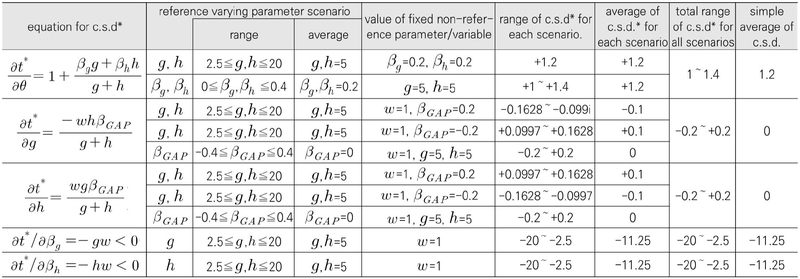
By simply plugging average values of parameters and normalized fixed values of variables, we can obtain the average values for the comparative static derivatives. The result is shown in the last column of <Table 1>. In terms of absolute values, buyer’s market share (βh) and seller market share(βg) are the most influential parameters, where the average value of comparative static derivative with regard to βh, which is , and the average value of comparative static derivative with regard to seller’s concentration , , are -11.25. Among the five derivatives, the ones for elasticities have the smallest values. The simple averages of the comparative static derivative with regard to demand elasticity, , and the comparative static derivative with regard to supply elasticity, , are all zeroes. The simple average of the comparative static derivative with regard to unit external cost is 1.2, which is larger than the ones with regard to elasticities but smaller than the ones with regard to market shares.

Numerical Simulation Scenarios and Results
Numerical simulations are conducted to examine the distribution’s of the derivatives according to the changes of the reference varying parameters.
Regarding the comparative static derivative of optimal disposal charge rate with respect to the unit external cost , numerical simulation is conducted over the range of reference varying parameters for elasticity and market structure. For , we have two simulations with respect to elasticity related parameters (g and h) and market shares (βg and βh). By simulating the value of over the values of g (inverse of demand elasticity), and h (inverse of supply elasticity), which are varying from 2.5 to 20, while keeping βg=0.2 and βh=0.2, we get the result 1.2. By simulating the value of over the values of βg(seller’s average market share) and βh(buyer’s average market share), which are varying from 0 to 0.4, we get the result distributed between 1 and 1.4, with average of 1.2. The overall range of the simulated values for is between 1 and 1.4, and the average is 1.2, which is the same as the simple average. The simulation result is demonstrated with a three dimensional diagram in <Figure 2>.

Numerical Simulations Result for ∂t*∂θ=1+βgg+βhhg+h and over βg and βh with g=h=5
The simulations of optimal disposal charge rate regarding the inverse of elasticities are conducted keeping w=1, a normalized value and keeping βGAP= 0.2 or βGAP= - 0.2. Although the average value of βGAP is equal to zero, if we choose zero as the fixed value for βGAP, the simulation results for will be zero, which is meaningless, so we instead chose +0.2 and –0.2 for the fixed values of βGAP.
The comparative static derivative of optimal disposal charge rate regarding the inverse of demand elasticity is simulated over the values of g (inverse of demand elasticity) and h (inverse of supply elasticity), which are varying from 2.5 to 20, while keeping w=1 and βGAP=0.2, we get the result between -0.1628 and –0.0997 with the average of –0.1. The simulation result is demonstrated with a three dimensional diagram in <Figure 3>. The same one is simulated over the values of g (inverse of demand elasticity), and h (inverse of supply elasticity), which are varying from 2.5 to 20, while keeping w=1 and βGAP= - 0.2, we get the result between 0.0997 and 0.1628 with the average of +0.1. The simulation result is demonstrated with a three dimensional diagram in <Figure 4>.

Numerical Simulations Result for ∂t*∂g=-whβGAPg+h over g and h, with βGAP=+0.2

Numerical Simulations Result for ∂t*∂g=-whβGAPg+h over g and h, with βGAP=-0.2
The same one is simulated over the values of βGAP, which are varying from –0.4 to +0.4, while keeping w=1 and g=5 and h=5, we get the result between -0.2 and +0.2 with the average of zero. We get the result for between -0.2 and +0.2 with the average of zero.
The comparative static derivative of optimal charge rate regarding the inverse of supply elasticity is simulated over the values of g (inverse of demand elasticity), and h (inverse of supply elasticity), which are varying from 2.5 to 20, while keeping w=1 and βGAP=0.2, we get the result between 0.0997 and 0.1628 with the average of +0.1. The simulation result is demonstrated with a three dimensional diagram in <Figure 5>. The same one is simulated over the values of g (inverse of demand elasticity), and h (inverse of supply elasticity), which are varying from 2.5 to 20, while keeping w=1 and βGAP=-0.2, we get the result between –0.1628 and -0.0997 with the average of -0.1. The simulation result is demonstrated with a three dimensional diagram in <Figure 6>.

Numerical Simulations Result for ∂t*∂h=wgβGAPg+h over g and h, with βGAP=+0.2

Numerical Simulations Result for ∂t*∂h=wgβGAPg+h over g and h, with βGAP=-0.2
The same one is simulated over the values of βGAP, which are varying from –0.4 to +0.4, while keeping w=1 and g=5 and h=5. We get the result for between -0.2 and +0.2 with the average of zero.
The comparative static derivative of optimal charge rate regarding the seller’s market share is simulated over the values of g, which is varying from 2.5 to 20, while keeping w=1, we get the result distributed between –2.5 and -20, with average of –11.25. By simulating the comparative static derivative of optimal charge rate regarding the seller’s market share over the values of h, which is distributed between 2.5 and 20, we get the result distributed between -2.5 and -20, with average of -11.25.
Simulation results are summarized in the following <Table 1>.
4. Summary of the Numerical Simulations
Unit external cost is the only important factor in determining the disposal charge rate in a competitive market. In a competitive market, it is always true that t*=θ and =1. In an imperfectly competitive market, not only unit external cost determines the optimal charge rate, but elasticity and market structure also play key roles. But the relative importance of parameters is not clearly visible if we only look at the comparative statics results mathematically. It can be seen by conducting numerical simulations.
The followings are derived from the numerical simulations. In an imperfectly competitive market, the value of optimal disposal charge rate is smaller than in competitive markets. This relationship is manifested by the negative value of the comparative static derivative of optimal charge rate regarding market share, which dictates that the optimal charge rate will be smaller as the market structure becomes less competitive either in supply or demand side. As shown in the following <Table 2>, market structures has the largest impacts on t*(optimal disposal charge rate). Considering that the policy makers and practitioners usually do not take market structure into consideration in determining the disposal charge rate, this has a fairly important implication.
Summary of the Numerical Simulation Results
Although unit external cost is not the sole factor for the optimal charge rate in an imperfectly competitive market, it is still fairly important. The average value of comparative static derivative of optimal charge rate is 1.2, which is larger than the one in a competitive market (=1).
In an imperfectly competitive market, market elasticity has some but minor role, much smaller than the other parameters. The average values are zeroes. In addition, when the buyer and seller have symmetric market structures, including the case of perfect competition, elasticity has zero effect in optimal charge rate decisions.
Ⅳ. Conclusion, Policy Implications, and Suggestions for Future Studies
In a competitive market, the unit external cost is the only parameter that matters in determining the optimal disposal charge rate. However, in an imperfectly competitive market, optimal disposal charge rate is determined by not only the unit external cost but also elasticities and market structures. Based on the results from numerical simulations, in an imperfectly competitive market, among the three factors (market structure, elasticity, unit external cost), market structure is the most important. Unit external cost is still important, while elasticity is the least important.
In many environmental policy related issues, competitive markets are implicitly or explicitly assumed. In this situation, the optimal disposal charge rate should always be the unit external cost. In a real world, however, policy designers usually consider elasticity as one of the important factors in determining the charge rate. Why this happens? We can speculate that the reason may be the revenue maximizing instinct (or concern) of the bureaucrats. It is well known that there exists a trade-off between tax rate and elasticity in maximizing the tax revenue in a competitive market, which meas that lower elasticity increases revenue-maximizing (not social welfare maximizing) disposal charge rate. Another possible explanation is that policy practitioners are aware that elasticity matters in an imperfectly competitive market which is usually the case in reality. However, the result from this study showed that the sign of the values of and are indeterminate, which makes the conventional (actually revenue maximizing) decision rules obviously inappropriate. In some case, the sign of the and are in the opposite direction to the conventional decision rules. Therefore, the conventional decision rule based on elasticity is sub-optimal, or even welfare deteriorating because it directs the disposal charge rate to the wrong, sometimes opposite direction.
A remarkable finding of this study is that market structure is the most important in determining the optimal charge rate. Policy maker usually do not seriously consider market structure in determining the disposal charge rate for wastes. Decision rules without considering market structure are misleading and could be even harmful. Having information on the market structure is the most important in decision making with regard to the optimal disposal charge rate.
This study needs to be extended to a more realistic market specification. Waste treatment service industry is split into intermediate treatment and final treatment. Next study would be a model which considers explicitly considers the separation of these two industries. Another extension would be the modeling work which incorporates the two input-output related waste treatment services and imperfect competition, which could be the extension of the CGE models which consider waste service as one of the production factors, as used in Lee, Kim, Kim and Han (2020).
Acknowledgments
본 논문은 한국연구재단 중견연구자 지원사업의 지원을 받아 이루어졌다(과제번호: 2022S1A5A2A01047527). 본 논문과 연관된 초기 내용들이 GCET19 Conference (Madrid, Spain, September 28, 2018), EAERE (Seoul, Korea, August 21, 2021), 그리고 43rd EBES Conference (Madrid, Spain, April 12-14, 2023) 에서 발표된 바 있다.
Notes
REFERENCES
-
Appelbaum, E., 1982, “The estimation of the degree of oligopoly power,” J. Econometrics, 19, pp.287-299
[https://doi.org/10.1016/0304-4076(82)90006-9]

- Barnett, A. H., 1980, “The Pigovian tax rule under monopoly,” American Economic Review, 70(5), pp.1037-1041.
-
Baumol, W. J., 1995, “Environmental industries with substantial start-up costs as contributors to trade competitiveness,” Annual Review of Energy and Environment, 20(1), pp.71-81
[https://doi.org/10.1146/annurev.eg.20.110195.000443]
- Bovenberg, A. L. and L. H. Goulder, 1996, “Optimal environmental taxation in the presence of other taxes: general-equilibrium analyses,” American Economic Review, 86(4), pp.985-1000.
- Chung, C., 2017, “Industrial organization models and their applications in food and agricultural industries,” Unpublished lecture note in Korea University.
-
David, M. and B. Sinclair-Desgagné, 2005, “Environmental regulation and the eco-industry,” Journal of Regulatory Economics, 28(2), pp.141–155
[https://doi.org/10.1007/s11149-005-3106-8]
-
David, M., A. D. Nimubona, and B. Sinclair-Desgagné, 2011, “Emission taxes and the market for abatement goods and services,” Resource and Energy Economics, 33, pp.179–191
[https://doi.org/10.1016/j.reseneeco.2010.04.010]
- Feess, E. and G. Muehlheusser, 1999, “Strategic environmental policy, international trade, and the learning curve: the significance of the environmental industry,” Review of Economics, 50(2), pp.178–194.
-
Feess, E. and G. Muehlheusser, 2002, “Strategic environmental policy, clean technologies and the learning curve,” Environmental and Resource Economics, 23, pp.149–166
[https://doi.org/10.1023/A:1021249404533]
- Ji, I. and C. Chung, 2016, “Assessment of market power and cost efficiency effects in the U.S. beef packing industry,” Journal of Rural Development, 39(Special Issue), pp.35~58.
- Kaneko, R., 2009, Institutional Design of Industrial Waste Tax: Towards the Promotion of Transition to Circular Society and Regional Environmental Conservation (in Japanese), Tokyo, Hakuto Shobo, 2009 (金子林太郞, 2009, 「産業廢棄物稅の制度設計- 循環型社會の形成促進と地域環境の保全に向けて」, 東京, 白桃書房.)
- Kim, G. and Y. Chang, 2015, “Analysis on the effect of waste disposal charge on the quantity of disposal and revenue,” a section in Study on the Design and Operation of Charge System for the Transition to Circular Society: Part I (in Korean), Ministry of Environment.
- Kim, H. and J. Kim, 2002, “The study on the optimal environmental tax in the presence of taxation on capital,” KYUNG JE HAK YON GU, 50(2), pp.105-125(in Korean).
-
Lee, H., J. Kim, G. Kim and T. Han, 2020, “Raising waste disposal charge rate will alleviate the shortage in landfill capacity in Korea?: a recursive dynamic KLWR CGE model,” Journal of Environmental Policy and Administration, 28(1)(in Korean)
[https://doi.org/10.15301/jepa.2020.28.1.211]
- Lho, S., 2002, “The optimal environmental tax rates in the generalized utilitarian social welfare function,” Environmental and Resource Economics Review 11(4), pp.689-706 (in Korean).
-
Misiolek, W. S., 1980, “Effluent taxation in monopoly markets,” Journal of Environmental Economics and Management, 7, pp.103-107
[https://doi.org/10.1016/0095-0696(80)90012-1]
- Requate, T., 2005, “Environmental policy under imperfect competition - a survey,” Economics Working Paper No 2005-12, Kiel University, Department of Economics, Kiel.
-
Sandmo, A., 1975, “Optimal taxation in the presence of externalities,” The Swedish Journal of Economics, 77(1), pp.86-98
[https://doi.org/10.2307/3439329]
한택환: 현재 서경대학교 명예교수이자 환경통계정보연구소 대표이며 University of Utah에서 경제학 박사학위를 받았다. 최근의 주된 관심은 폐기물 처리 서비스 산업에 대한 이론적・정량적 분석을 통하여 바람직한 폐기물 정책의 대안을 제시하는 것이다(twhan@skuniv.ac.kr).