[ Article ]

Journal of Environmental Policy and Administration - Vol. 28, No. 1, pp.143-162

ISSN: 1598-835X (Print) 2714-0601 (Online)

Print publication date 31 Mar 2020

Received 02 Feb 2020 Revised 06 Feb 2020 Accepted 26 Feb 2020

DOI: https://doi.org/10.15301/jepa.2020.28.1.143

The Impact of the Diesel Tax Reform on Air Pollutant Emissions in Korea Using a Time-Varying Parameter Model

Byung Min Soon^** ; Dong Won Shin^*** ; Seung Yub Lee^****

**First Author, Research Fellow, Korea Rural Economic Institute.
***Corresponding Author, Research Fellow, Korea Environment Institute.
****Co-author, Researcher, Missouri Department of Health and Senior Service, USA

시간가변계수 모형을 적용한 대기오염물질에 대한 경유세 인상 효과

순병민^** ; 신동원^*** ; 이승엽^****

Abstract

This study examines the impact of the increase in the diesel tax on air pollution reduction using a constant elasticity of substitution (CES) function. A time-varying parameter model is used to vary the elasticity of substitution between diesel and gasoline over time. The result s showed that diesel and gasoline were strongly substituted from 2013 to 2017, but their substitution was weaker in 2018. In a scenario in which the diesel tax increased by 40%, diesel consumption decreased by 2,308 thousand tons. In terms of air pollutant emissions, nitrogen oxide, CO, and PM_2.5 decreased by 50,501tons, 8,495 tons, and 1,268 tons, respectively. These results provide policy suggestions for reducing air pollutant emissions and encouraging environmentally friendly vehicles.

초록

본 연구는 경유세 인상이 대기오염물질 저감효과가 있는지 CES 함수를 통해 나타낸다. 또한 시간가변계수(Time-varying parameter)를 함수에 포함시킴으로써 시간의 흐름에 따른 경유와 휘발유의 대체관계를 나타낸다. 그 결과 2013년부터 2017년까지 경유와 휘발유의 대체관계가 높았다가 2018년 두 연료의 대체관계는 다소 작아진 것으로 나타났다. 경유세 40% 인상 시나리오 분석 결과, 전체 경유 소비량의 10%인 230만 톤의 경유 소비량이 한 해 동안 감소하는 것으로 나타났다. 대기오염물질은 질소산화물(NO_x) 5만톤, 일산화탄소(CO) 8천톤, PM_2.5 1천톤이 감소하는 것으로 나타났다. 본 연구 결과는 대기오염물질 저감 정책 및 친환경 자동차 전환 정책에 도움이 될 수 있다.

Keywords:

Diesel Tax, Emission Reduction Policy, Time-Varying Parameter, NO_x, CO, PM_2.5

키워드:

경유세, 배출저감정책, 시간가변계수, 질소산화물, 일산화탄소, PM_2.5

I. Introduction

South Korea has serious air pollution problem. One of factors increasing air pollution is from diesel uses (Shin et al., 2019). Air pollutants such as PM_2.5 and NO_x from vehicle using diesel is about 70% among air pollutants from all vehicles (National Air Pollutants Emission Service, 2019). Recently, the increase in diesel tax is proposed to reduce air pollution. The average price ratio of gasoline to diesel in the EU is 1.09 in 2018 (European Automobile Manufacturers Association, 2019). The price of gasoline relative to diesel in Korea is 1.11 in December 2018, indicating that the diesel price in Korea is lower relative to in the EU. In the case of the tax ratio of gasoline to diesel in EU members, Germany is 1.39, France is 1.20, and the UK is 1.00. Most of the tax ratio in the EU is lower than the tax ratio, 1.41, in Korea. The price and tax ratios in Korea and the EU can provide policy implication that it is likely to increase diesel tax. South Korea’s government also consider increasing diesel tax to reduce air pollution. Therefore, it is necessary to analysis how much raising diesel tax reduces air pollutant emissions.

Various empirical economic studies related energy broadly use a constant elasticity of substitution (CES) function. For equilibrium models, a global trade analysis projection (GTAP) uses the CES function that is called an Armington function (Hertel and Tsigas, 1997; Armington, 1969). The Armington function generates the elasticity of substitution and the country of origin bias in the import section. Moreover, GTAP-E is developed to study CO2 emission and the greenhouse effect (Truong, 2007). A common agricultural policy regionalized impact (CAPRI) analysis developed by the University of Bonn develops a multi-commodity model based on CES function (Britz, 2008). The CES function is used to estimate the elasticity of substitution in the energy field. Kemfert (1998) estimates the elasticity of substitution between capital, energy, and labor for the German industry using a nest CES production function. Zha and Zhou (2014) use CES function to estimate the elasticity of substitution between energy and non-energy for the Chinese industrial sectors. Therefore, we use the CES function to estimate the elasticity of substitution between diesel and gasoline.

One possible question might be whether the estimated elasticity of substitution are fixed. Traditional estimation methods generate fixed estimates. However, actual estimates can fluctuate over time if unobserved factors tend to vary over time (Becker, Enders and Hurn, 2005). Lim (2019) estimates the city gas demand in Korea using a Kalman filter method to vary price and income elasticities over time. The results show that a Kalman filter method generates more accurate information. However, the Kalman filter model requires a specific functional form and priors from expert knowledge (Harvey, 1989). Depending on functional form or priors, the results could be changed. To avoid selecting a specific functional form and priors, Chang et al. (2014) estimate electricity demands in Korea using a smooth time-varying coefficient cointegration approach by a flexible Fourier functional form. Park and Zhao (2010) estimate U.S. gasoline demand using a smooth time-varying cointegration approach. These authors use a different method to vary parameters over time, but emphasize that actual estimates can fluctuate over time.

The objective of our study is to examine the impact of diesel tax on air pollutant emissions in Korea. We set the CES utility functional form to estimate the elasticity of substitution and impose a flexible Fourier functional form to vary a key parameter over time. To the best of our knowledge, we use the Fourier series approximation to estimate the elasticity of substitution between gasoline and diesel in Korea. Using the time-varying elasticity of substitution, we then simulate a scenario what air pollutant emissions would be if the diesel tax increases by 40%. The 40% increase in the diesel tax makes that the ratio of tax between diesel and gasoline is almost one and the ratio of price is 1.07 that is similar to ratio in the EU.

The article is structured as follows. The following section introduces the empirical method. The data is in the third section. The fourth section represents the results in terms of model results and experiment results. The last section summarizes our findings and draws some conclusions.

Ⅱ. Empirical Method

1. Demand Equation

A CES utility function is used to estimate the elasticity of substitution. CES utility function is assumed to be weakly separable in the types of fuel. In our representation, consumers can choose between gasoline and diesel. The utility function is represented as follows:

U G, D = δ ⋅ G σ - 1 σ + 1 - δ ⋅ D σ - 1 σ σ σ - 1 s u b j e c t t o G ⋅ P G + T G + D ⋅ P D + T D = I

(1)

where G and D represent gasoline and diesel consumption, respectively. Prices at the pump for gasoline and diesel consist of price without tax, P_G for gasoline and P_D for diesel, and tax, T_G and T_D . Since CES utility function is separable from consumption of other commodity, changes in fuel consumption do not affect other consumption. σ represents the elasticity of substitution between gasoline and diesel.

The demand equations can be derived through an optimization process. As following the first-order condition, we derive the demand equation as follows:

G D = δ 1 - δ σ P D + T D P G + T G σ

(2)

The ratio of gasoline to diesel consumption is determined by the ratio of prices at the pump of diesel to gasoline. Taking the logarithms, the demand equation becomes

log ⁡ G D = σ ⋅ log ⁡ δ 1 - δ + σ ⋅ log ⁡ P D + T D P G + T G

(3)

The equation is consequently

y t = β 0 + β 1 p t + ε t

(4)

where (4.1) y_t = log (G/D) , (4.2) β₀ = σlog (δ/(1 - δ)) , (4.3) β₁ = σ, (4.4)p_t = log ((P_D + T_D )/(P_G + T_G)).

2. Time-Varying Parameter Model

Unknown factors are likely to cause parameters to fluctuate over time. For example, seasonality and unexpected oil shock can change parameters. Hence, our study is designed to vary parameters with a function of time as a proxy variable for unobservable factors. A Fourier-series approximation is used to vary parameters (Becker, Enders and Hurn, 2005; Chang et al., 2014; Park and Zhao, 2010). An approach developed by Soon and Thompson (2019) is applied to impose a trigonometric function on β₁ in Equation (4) as a function of time. With the time-varying elasticity of substitution, β₁ , the model can have time-varying parameters as follows:

y t = β 0 + β 1, t p t + ∑ i = 1 11 γ i M i + ε t

(5)

where β_1,t = β (t/T) , t represents the period with T as the total number of observation. M_t is monthly dummy variables. To make β_1,t a function of time, we use a Fourier-series approximation as follows:

β 1, t = λ 0 + λ 1 sin ⁡ 2 π t T λ 2 cos ⁡ 2 π t T + λ 3 sin ⁡ 4 π t T + λ 4 cos ⁡ 4 π t T

(6)

We estimate two sin and cos frequencies so that β_1,t approximates the changing parameter of consumer utility and demand. Imposing Equation (6) into Equation (5), the demand equation becomes

y t = β 0 + λ 0 p t + λ 1 sin ⁡ 2 π t T p t + λ 2 cos ⁡ 2 π t T p t + λ 3 sin ⁡ 4 π t T p t + λ 4 cos ⁡ 4 π t T p t + ∑ i = 1 11 γ i M i + ε t

(7)

We conduct a linear function with new variables to approximate the non-linear function given by Equation (7). Finally, our linear functional form is given by

y t = β 0 + λ 0 p t + λ 1 p t, s i n 1 + λ 2 p t, c o s 1 + λ 3 p t, s i n 2 + λ 4 p t, c o s 2 + ∑ i = 1 11 γ i M i + ε t

(8)

where (8.1) $p t, s i n 1 = sin ⁡ 2 π t T p t$ , (8.2) $p t, c o s 1 = cos ⁡ 2 π t T p t$ , (8.3) $p t, s i n 2 = sin ⁡ 4 π t T p t$ , and (8.4) $p t, c o s 2 = cos ⁡ 4 π t T p t$ . We then estimate λ_i for i = 0 to 4 in Equation (8). If $λ 1^= λ 2^= λ 3^= λ 4^= 0$ , then the TVP model shrink to the fixed parameter model. If not, then we get time-varying elasticity of substitution, β_1,t , with estimated $λ i^≠ 0$ for 1, 2, 3, or 4 (Chang et al., 2014).

3. Experiment Approach

We conduct an experiment to examine the impact of the diesel tax on diesel consumption. To do that, we estimate time-varying parameter values up to the period we observed. Time-varying parameter estimates in that period, $β 1, t = β t T + h$ , are extended to forecast parameter values for the future period, $β 1, t = β t + h T + h$ , where h is the future period. Here, we forecast diesel demand for one year, which h is 12. The forecast parameter values is used to estimate diesel demand quantities for one year.

We assume that gasoline and diesel prices in the future year is the price in the last observation for the baseline. For the scenario that diesel tax is increased by 40%, we add the diesel tax into diesel price that we use for the baseline. We choose 40% of the increase in diesel tax because the ratio of diesel to gasoline tax is close to one. We then compare the estimate of diesel demand between the baseline and scenario results.

We calculate how much air pollution emissions could be reduced per year based on the increased diesel tax for CO, NOx, and PM2.5.

E = D × E F

(9)

where E and D represent emissions and diesel consumption, respectively. EF is emission factor that is related to the quantity of each pollutant released to the air with diesel use. These factors are calculated as the weight of pollutant divided by a unit volume of diesel from the recent emission data (USEPA, 2019; National Air Pollutant Emission Service, 2019).

Ⅲ. Data

Monthly gasoline and diesel consumption and prices from January 2000 to December 2018 are used. Consumption data are obtained from Korea Energy Economics Institute. Price data are consisted of the price without fuel tax, fuel tax, value-added tax, and the price at the pump and obtained from Opinet developed by Korea National Oil Corporation.²⁾ Pollutant emission data are gathered from National Air Pollutant Emission Service and the most recent available data is 2016.

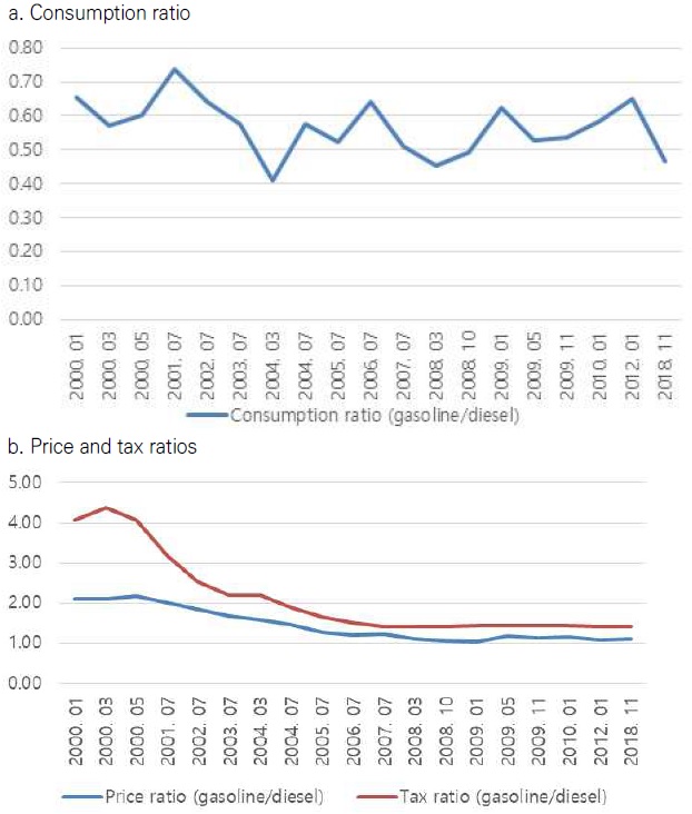
<Figure 1> shows the historical gasoline and diesel consumption and price ratios. Figure 1.a. shows that Diesel consumption has been larger than the gasoline price as the ratio of gasoline to diesel consumption is less than 1. Diesel consumption falls sharply in 2012 because of diesel scandal that air pollution emission of Volkswagen is miscalculated. This diesel emission scandal results in a reduction in Volkswagen diesel cars and an increase in distrust of diesel car that people believed it as environmentally friendly car. Overall, diesel consumption in Korea is about 63% in 2018 among total fuel consumption.

Consumption, price and tax ratioSource: Korea Energy Economics Institute, Korean National Oil Corporation

Figure 1.b. indicates that the ratio of diesel to gasoline. The diesel price at the pump has been increased, implying that the ratio of diesel to gasoline is close to one. However, comparing the ratio of diesel to the gasoline tax, the ratio is much lower than one and below the ratio taking the price at the pump into account, implying that diesel tax is lower. If the diesel tax rate is increased, then the diesel price at the pump is likely to be above the gasoline price at the pump.

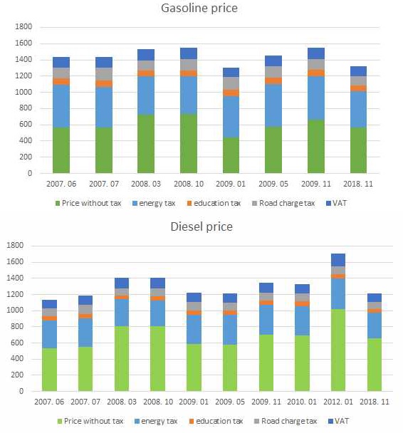
Diesel tax, especially energy tax, is lower than gasoline tax <Figure 2>. The diesel price without tax is higher than the gasoline price, but after tax, the diesel price at the pump is lower than the gasoline price. This lower diesel price can lead to an increase in diesel consumption. This implication is based on the model results, even though other factors such as the increase in the use of SUV vehicles can results in the increase in diesel consumption.

Fuel taxSource: Korean National Oil Corporation

Ⅳ. Results

1. Model Results

We first explore the fixed parameter model estimation. <Table 1> shows that the fixed parameter model generates statistically significant parameter estimates. The elasticity of substitution between gasoline and diesel is 0.19 and statistically significant at the 5% level. D98 and D08 are dummy variables for the IMF crisis in 1998 and financial crisis in 2008, respectively. The R-square and the adjusted R-square are 0.43 and 0.40, respectively. The results of the fixed parameter model can be reliable. However, the fixed parameter model cannot show that actual elasticity of substitution can fluctuate over time if various factors affect parameters and tend to vary over time (Becker, Enders and Hurn, 2005).

Fixed parameter model estimates

Comparing to the fixed parameter model estimate, the TVP model results can be more reliable and are used to estimate diesel demand by the diesel policy change. <Table 2> illustrates the coefficients. λ_i for i=0 to 6 are coefficient for variables including sin and cos frequencies. Monthly dummy variables from January to November are used to capture the seasonal effect of gasoline and diesel demand (Kawashima and Sari, 2010). The R-square and the adjusted R-square are 0.62 and 0.58, respectively. These R-square in the TVP model is greater than the value in the fixed parameter model, implying that the TVP model fits well relative to the fixed parameter model. F-statistic shows that we can reject the null hypothesis, which all λ_i are equal to zero. Especially, λ₀ , λ₁ , λ₂ , and λ₆ are statistically significant, implying that they are not equal to zero. These coefficients are used to estimate the time-varying elasticity of substitution between gasoline and diesel.

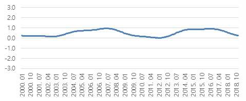
Time-varying parameter model estimates

Based on TVP estimates, we can calculate time-varying elasticity of substitution in equation 6. <Figure 3> shows the elasticity of substitution between gasoline and diesel over time. From 2013 to 2017, the elasticity of substitution is high, implying that gasoline and diesel are strongly substituted. Then, after early 2018, they are less substituted. The results imply that the change in the relative price is likely to change fuel consumption during the period from 2013 to 2017 because the elasticity of substitution is high. After then, the changes in the relative price does not cause fuel consumption as much as the change in fuel consumption from 2013 to 2017 because the elasticity of substitution is relatively lower to pre-2018. One of possible reasons is that fuel consumers can concern of increasing fine dust generated by diesel cars. The TVP model shows the time-varying elasticity of substitution over time that the fixed parameter model cannot generate.

Time-varying elasticity of substitutionSource: authors’ calculations

2. Scenario Results

We conduct a scenario that diesel tax is increased by 40%. Recently, Korea government announces that they consider increasing diesel tax by 40% to reduce air pollution emissions. The increase in diesel tax by 40% makes the ratio of diesel to gasoline tax close to one. The tax increase by 40% also might be reasonable if we compare the EU and U.S. air pollution policy in terms of the diesel tax regime. We estimate the potential reduction of diesel consumption and air pollutant emissions by diesel tax policy change.

There are several assumptions to simulate the scenario. The gasoline and diesel prices are assumed to be the price at the last observation period. The model here uses the prices in 2018 December. The total consumption of gasoline and diesel is constant, which the change in the relative price does not cause the total consumption. We presume that vehicle types are not taken into account.

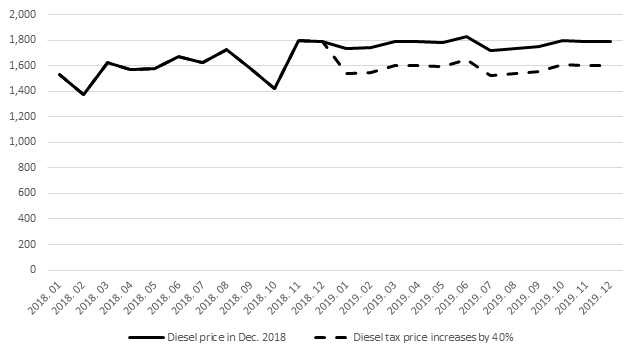
We impose 40% of tax into diesel price to examine how much diesel consumption decreases based on estimated parameters <Figure 4>. The monthly average reduction in diesel consumption is about 192 thousand tons. The increase in the diesel tax by 40% reduces 2,308 thousand tons per year, illustrating that 10% of diesel consumption is reduced a year. The decrease in diesel consumption by the increase of the diesel tax might affect gasoline and diesel prices. However, as we mentioned before, fuel prices are not changed as exogenous. The time-varying elasticity of substitution we estimate causes the fluctuation of diesel consumption for the projected year.

Diesel consumption by 40% diesel tax increase (thousand tons)Source: authors’ calculations

<Table 3> shows calculated values of emission reduction due to the diesel tax. Nitrogen oxide is the largest pollutant from diesel and 50,501 ton of NO_x can be reduced. Also, reduction of diesel use can decrease emission of CO and PM_2.5 by 8,495 and 1,268 ton, respectively. By the construction, all amount of pollutant emission is reduced about 10%. We calculate social benefit (reduced social costs) based on Ministry of Environment of Korea (as cited in Kang et al., 2016). It shows NO_x is the most reduction of social costs with more than 2 million won. Social cost reduction of PM_2.5 is 0.6 million in respect of urban area.

Air pollution reduction by 40% diesel tax increase

Ⅴ. Conclusions

The diesel use for vehicles can generate air pollution as well as the gasoline use. Recently, old vehicles using diesel seriously increase air pollutant emission in Korea. Therefore, energy policy, which increases diesel tax, is proposed to decrease the diesel use and encourage to increase the use of electric car. Our study is to examine the impact of diesel tax on air pollutant emissions. The CES function is used to estimate the elasticity of substitution between diesel and gasoline. Since we assume that the elasticity of substitution is not fixed, we vary that estimate over time using the Fourier-series approximation. Given estimate results, we make scenario results.

The result indicates that diesel and gasoline are strongly substituted from 2013 to 2017. In 2018, the substitution between diesel and gasoline are weaker. The possible reasons are that the gap between diesel and gasoline is smaller and the policy for electric and hybrid cars is instituted. The results imply that recent energy policy change that imposes tax into diesel use less causes to diesel consumption relative to pre-2018. This time-varying parameter model demonstrates how the estimates move over time that the fixed parameter model cannot generate.

The increase of diesel tax by 40% results in the decrease of diesel use by 2,308 thousand tons. Given estimate results that we use the time-varying parameter model and price ratio and consumption in 2018, we estimate the impact of 40% diesel tax increase on not only diesel consumption but also air pollutant emission. Based on air pollutant emission factor gathered from National Air Pollutant Emission Service (2019), NO_x, CO, and PM_2.5 reduced by 50,501, 8,495, and 1,268 tons, respectively. These amount is about 10% of total air pollutant emission before tax. In addition, social benefits (reduced social costs) of reduced pollutants are 2.4 million (NO_x), 0.2 million (CO) and 0.6 million (PM_2.5).

There are some limitations. We assume that the historical price and consumption ratios are used to estimate our scenario. If we endogenize the price in the model, then we can estimate our scenario more approximately. We refer to emission factor assumed that all diesel uses generate the same air pollutant emission, even though air pollutant emission can be different depending on vehicle type. However, our study shows the amount of reduction in diesel consumption and air pollutant emission by 40% diesel tax increase based on economic theory and the TVP. These results suggest that the government is likely to make a policy that increases the use of electric car and hydrogen fueled car, and provides infrastructures for electric car. Hence, this approach helps policy makers or applied economists who want to estimate air pollutant emission.

Acknowledgments

This work was supported by Korea Environment Institute as 「A study on Enhancing social Acceptance of Tax Reform for Conversion of Transport Energy (WO 2018-11)」 and 「Collaborative research on the green economy (GP2020-15)」.

Notes

2) Opinet, http://www.opinet.co.kr/user/main/mainView.do.

References

Armington, P. S., 1969, “A theory of demand for products distinguished by place of production,” Staff Papers (International Monetary Fund ), 16(1), pp.159-178. [https://doi.org/10.2307/3866403]
Becker, R., W. Enders, and S. Hurn, 2006, “Modeling inflation and money demand using a Fourier-Series approximation,” Contributions to Economic Analysis, 276, pp.221-246. [https://doi.org/10.1016/S0573-8555(05)76009-0]
Britz, W., 2008, “Automated model linkages: The example of CAPRI,” German Journal of Agricultural Economics, 57, pp.363-367. [https://doi.org/10.22004/ag.econ.97707]
Chang, Y., C. S. Kim, J. I. Miller, J. Y. Park, and S. Park, 2014, “Time-varying long-run income and output elasticities of electricity demand with an application to Korea,” Energy Economics, 46, pp.334-347. [https://doi.org/10.1016/j.eneco.2014.10.003]
European Automobile Manufacturers Association, 2019, ACEA tax guide, Brussels: ACEA, Retrieved from https://www.acea.be/uploads/news_documents/ACEA_Tax_Guide_2019.pdf, .
Harvey, C. R., 1989, “Time-varying conditional covariances in tests of asset pricing models,” Journal of Financial Economics, 24(2), pp.289-317. [https://doi.org/10.1016/0304-405X(89)90049-4]
Hertel, T. W. and M. E. Tsigas, 1997, Structure of GTAP, In T. W. Hertel (ed.), Global trade analysis: Modeling and applications, (pp.13-73), Cambridge: Cambridge University Press. [https://doi.org/10.1017/CBO9781139174688.003]
Kang, K. K., J. S. Hahn, E. J. Seo, and K. R. Cho, 2016, Social costs caused by excessive emission of air pollutants from EURO-5 diesel passenger vehicles on the road, (Policy report; 2016-08), Sejong: Korea Environmental Institute.
Kawashima, S. and D. A. Sari, 2010, “Time‐varying Armington elasticity and country-of‐origin bias: From the dynamic perspective of the Japanese demand for beef imports,” Australian Journal of Agricultural and Resource Economics, 54(1), pp.27-41. [https://doi.org/10.1111/j.1467-8489.2009.00477.x]
Kemfert, C., 1998, “Estimated substitution elasticities of a nested CES production function approach for Germany,” Energy Economics, 20(3), pp.249-264. [https://doi.org/10.1016/S0140-9883(97)00014-5]
Lim, C., 2019, “Estimating residential and industrial city gas demand function in the Republic of Korea—A kalman filter application,” Sustainability, 11(5), 1363. [https://doi.org/10.3390/su11051363]
National Air Pollutant Emission Service, 2019, 2016 national emission of air pollution statistics, Brussels: Europa EU.
Park, S. Y. and G. Zhao, 2010, “An estimation of US gasoline demand: A smooth time-varying cointegration approach,” Energy Economics, 32(1), pp.110-120. [https://doi.org/10.1016/j.eneco.2009.10.002]
Shin, D. W., C. H. Lee, J. S. Hahn, D. W. Jung, Y. M. Chung, and B. M. Min, 2019, A study on enhancing social acceptance of tax reform for conversion of transport evergy, (KEI Policy report; 2019-07), Sejong: Korea Environmental Institute.
Soon, B. M. and W. Thompson, 2019, “Japanese beef trade impact from BSE using a time‐varying Armington model,” Agribusiness, pp.1-17. [https://doi.org/10.1002/agr.21631]
Truong, T. P., 2007, GTAP-E: An energy-Environmental version of the GTAP model with emission trading-USER’S GUIDE, GTAP resource, 2509, https://www.gtap.agecon.purdue.edu/resources/download/3552.pdf, .
Zha, D. and D. Zhou, 2014, “The elasticity of substitution and the way of nesting CES production function with emphasis on energy input,” Applied Energy, 130, pp.793-798. [https://doi.org/10.1016/j.apenergy.2014.01.093]
Korea Energy Economics Institute, https://www.keei.re.kr/main.nsf, .
Korea National Oil Corporation, https://www.knoc.co.kr, .
Opinet, http://www.opinet.co.kr/user/main/mainView.do, .
United States Environmental Protection Agency (USEPA), 2019, “Basic information of air emissions factors and quantification,” https://www.epa.gov/airemissions-factors-and-quantification/basic-information-air-emissionsfactors-and-quantification, , [2019.5.5]

Byung Min Soon is a research fellow at the Korea Rural Economic Institute (KREI). He received a Ph.D. in Agricultural and Applied Economics from the University of Missouri. His primary research focuses on environmental policy analysis, international trade, and price analysis (soonbm@krei.re.kr).

Dong Won Shin is a research fellow at the Korea Environment Institute (KEI). He received a Ph.D. in Agricultural and Applied Economics at the University of Missouri. The main areas of interest are environmental policy in air pollution, technology and innovation adoption, behavioral economics, consumer science (dwshin@kei.re.kr).

Seung Yub Lee is a research analyst III at the Missouri Department of Health and Senior Service. He received a Ph.D. in Agricultural & Applied Economics from the University of Missouri. The main areas of interest are adoption of practices and policy related to environmental quality and policy analysis (slb66@mail.missouri.edu).

Variables	Values
Note: , , and **denote significant at the 10%, 5%, and 1% levels
β₀	-0.66***
β₁	0.19**
D98	0.21**
D08	0.02
$β 0 β 1$	-3.47
R²	0.43
ADj.R²	0.40

Variables	Values	Variables	Values
Note: , , and **denote significant at the 10%, 5%, and 1% levels
β₀	-0.59***	Jan	0.09***
λ₀	0.49***	Feb	0.09***
λ₁	-0.39***	Mar	0.01
λ₂	-0.13*	Apr	0.01
λ₃	0.05	May	0.02
λ₄	-0.04	Jun	-0.07**
λ₅	0.01	Jul	0.12***
λ₆	-0.07**	Aug	0.10***
D98	0.15**	Sep	0.07**
D08	-0.02	Oct	-0.01
		Nov	0.01
R²	0.62	F-statistics	7.55***
ADj.R²	0.58

	Emission factor (ton/toe)	Emission (ton)		Reduction (ton)	Social benefit (1,000 won2018)
	Emission factor (ton/toe)	Before tax	After tax	Reduction (ton)	Social benefit (1,000 won2018)
Note: Social costs (won/ton) from Kang et al. (2016) Source: authors’ calculations
NO_x	21.88	465,056	414,555	50,501	2,424
CO	3.68	78,226	69,731	8,495	246
PM_2.5	0.51	11,673	10,405	1,268	597